12/8/00
In this experiment, we examined packets from trace6.tsh. For the first part of the experiment, we compared the number of TCP to UDP packets. We also calculated the relative bandwidth used by each protocol. In the second half of the experiment, we isolated Telnet packets and recorded their number of sessions in the trace, average length, throughput, number of packets, interarrival time, and bandwidth. We chose to analyze Telnet sessions because the trace showed a reasonable amount of packets.
We implemented the packet
analyzer by reading in the packets from the file into a structure. First we needed to retrieve the start and
finish times of the trace in order to determine the interval size, so we
scanned through the file and found the earliest and latest packet. After dividing the trace into intervals, we
scan through the trace file once again and get each packet.
Each packet is then passed
to two functions, one tabulates the TCP, UDP length and packet count
information for part 5 of the project.
Another function analyzes the packet to determine if it belonged to a
previously created session. In the case
that the packet's addresses and ports matches up with one of the sessions, we
would take that packet to be part of the session and add the information to the
session information. Otherwise we would
create a new session and place the packet information in the new session.
To keep track of all this
information, we had a session link-list, which recorded all of the sessions
over the trace, and we also had an interval array. Inside this interval array, there are two link lists and a size
variable. The size keeps track of bytes
sent by the particular application we are analyzing, and the first link list is
a list of pointers to sessions that are found in this interval. These pointers point to a particular session
from the main session list. The second
link list keeps track of session information in each individual interval
separately. We also had an array of the
TCP and UDP information for the 20 intervals that we split the trace into.
At the end of the program we
summarize all the information and print out the corresponding tables into a
comma separated value (.csv) file. We
traverse the appropriate lists and arrays and gather sums and averages to
obtain our values. After we are done,
we had to release all the memory we used in dynamically allocating these link
lists, so we would not have a memory leak.
We also added the functionality of displaying when each SYN and FIN is
encountered during the debug phase. We
were concerned with the results of our data so we implemented this feature, but
we disabled it in the final revision of the program. More details pertaining the individual sections is mentioned in
the explanation of the charts and graphs.
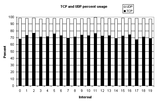
In the first part of this section, we were asked to find the percentage of TCP packets and UDP packets that were observed for each interval and for the lifetime of the trace. In order to accomplish this, we scanned through the trace file and extracted each packet. For each interval, we examined the protocol field in order to determine whether it was a TCP or UDP packet. A protocol value of 17 utilizes UDP, and a protocol of 6 utilizes TCP.
Figure 1 below depicts the percentage of TCP packets versus UDP packets. The lifetime of the trace was divided into twenty intervals of 47.392 msec. Our trace data began at 13.48 seconds.
|
TCP Traffic % vs UDP Traffic % |
||
|
Start = 13483164 us |
|
|
|
Interval |
TCP
Traffic |
UDP
Traffic |
|
0 |
68.3049 |
30.4915 |
|
1 |
73.6458 |
24.6875 |
|
2 |
76.6816 |
22.1973 |
|
3 |
71.0881 |
26.4249 |
|
4 |
71.9372 |
26.0733 |
|
5 |
75.5827 |
22.4195 |
|
6 |
72.9187 |
24.7847 |
|
7 |
69.4301 |
28.3938 |
|
8 |
71.3212 |
26.5306 |
|
9 |
74.2009 |
23.7443 |
|
10 |
72.9332 |
25.2548 |
|
11 |
76.1749 |
23.1694 |
|
12 |
72.4458 |
26.4190 |
|
13 |
73.1557 |
25.0000 |
|
14 |
69.0476 |
28.8961 |
|
15 |
72.6154 |
25.9487 |
|
16 |
74.4235 |
24.0042 |
|
17 |
67.1488 |
30.8884 |
|
18 |
71.3195 |
26.7176 |
|
19 |
69.2703 |
28.1603 |
|
LifeTime |
72.1307 |
26.0532 |
Figure 1
We notice from this graph that TCP traffic greater than UDP traffic, almost three times as much. This concurs with our expectations. Due to the reliability of TCP, it is a more widely used protocol in the transport layer. Also, we can discern from the graph that TCP and UDP traffic comprise almost 100% of the total traffic in this trace.
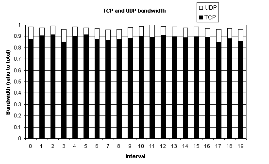
Next,
we analyzed the relative bandwidth used by TCP and UDP over each interval. The length of each payload and header was
recorded for each interval. This value
was then divided by the duration of the interval to obtain the relative
bandwidth. The TCP versus UDP relative
bandwidth is illustrated in Figure 2.
|
TCP vs |
UDP |
|
|
Interval |
TCP Bandwidth |
UDP Bandwidth |
|
0 |
0.875294 |
0.109114 |
|
1 |
0.906585 |
0.068848 |
|
2 |
0.913934 |
0.078371 |
|
3 |
0.852351 |
0.111287 |
|
4 |
0.903826 |
0.077761 |
|
5 |
0.914153 |
0.060518 |
|
6 |
0.87415 |
0.097495 |
|
7 |
0.869298 |
0.089043 |
|
8 |
0.874316 |
0.089351 |
|
9 |
0.883673 |
0.096451 |
|
10 |
0.901542 |
0.087269 |
|
11 |
0.894476 |
0.103487 |
|
12 |
0.912137 |
0.073707 |
|
13 |
0.899152 |
0.085444 |
|
14 |
0.889082 |
0.086295 |
|
15 |
0.896308 |
0.085271 |
|
16 |
0.89449 |
0.074975 |
|
17 |
0.845996 |
0.116869 |
|
18 |
0.881236 |
0.087919 |
|
19 |
0.860014 |
0.103012 |
|
Lifetime Bandwidth |
0.88695 |
0.08924 |
Figure 2
The
relative bandwidth of TCP data stays consistently around 90%, compared with UDP
data, which is only about 10% relative to total traffic. Hence, this experiment shows that TCP has
much higher relative bandwidth than UDP.
Over the entire trace lifetime, we see that the TCP data takes up ten
times more bandwidth than UDP data.
For the next part of the project, we chose to analyze Telnet sessions. This was completed by isolating all packets with a source or destination port of 23.
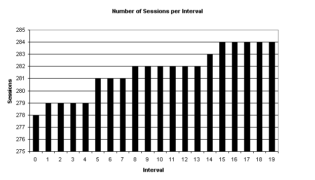
To isolate the number of sessions, we compared the port numbers and also the source and destination addresses. Whenever packets had matching port and IP addresses, we interpreted the packets to be part of the same session. A histogram of the results from this experiment are shown below in Figure 3.
|
Interval |
Sessions |
|
0 |
|
|
1 |
279 |
|
2 |
279 |
|
3 |
279 |
|
4 |
279 |
|
5 |
281 |
|
6 |
281 |
|
7 |
281 |
|
8 |
282 |
|
9 |
282 |
|
10 |
282 |
|
11 |
282 |
|
12 |
282 |
|
13 |
282 |
|
14 |
283 |
|
15 |
284 |
|
16 |
284 |
|
17 |
284 |
|
18 |
284 |
|
19 |
284 |
Figure 3
Once again, the lifetime of the trace was divided
into 20 intervals. Then, we recorded
the number of sessions open during each interval. Whenever a packet with a new pair of source and destination
addresses was seen, a new session was added to the interval. When a packet arrived with FIN=1, the session
was closed and removed from the total number of sessions. As can be observed from the graph above,
more sessions are opened than are closed in this trace. This is reasonable because many packets from
different sessions can go through this router, but not all of the FIN packets
of each session may go through the same router. The total number of sessions over the trace lifetime was 284.
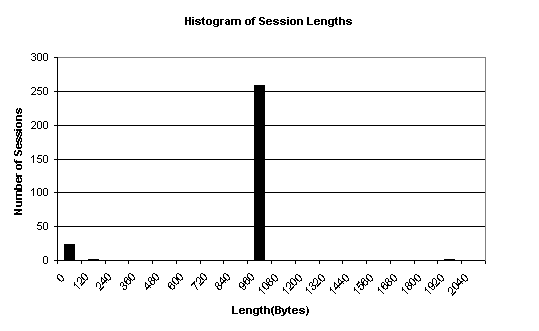
The average session length was also recorded. For each sessions’ packets, the length field was analyzed and saved. To find the average length of a session, the packets in a session were added together and then divided by the number of total packets in that session. Figure 4 depicts a histogram of session lengths.
|
# sessions |
|
|
6 |
4 |
|
3 |
5 |
|
1 |
6 |
|
7 |
8 |
|
1 |
9 |
|
2 |
10 |
|
1 |
11 |
|
1 |
12 |
|
1 |
16 |
|
1 |
125 |
|
259 |
1016 |
|
1 |
2032 |
Figure 4.
From the figure above, we observe that a majority of
the sessions exchanged 1016 bytes of data.
This standard size is most likely from sending a screenful of data from
the host to the server. Many sessions
also exchanged less than 20 bytes of data.
This may be from sending small prompts or the user typing characters.
We
next measured the session throughput.
Throughtput is the total amount of data transferred by a session
excluding overhead. To calculate this,
we summed up the lengths of the packets in each session. 36 bits were subtracted from each packet to
exclude packet headers. Then this
amount was divided by the duration of the session. The time for each session was calculated using the following
method. For each session, the timestamp
of the packets with SYN and FIN bits on were saved. If a session was detected that did not begin with a SYN bit equal
to one, the first packet of this session probably existed earlier before this
trace6 or the first packet did not go through this router. When this occurs, we take the start time to
be the beginning time of the trace. We
have a similar procedure for those sessions that do not have a packet where FIN
is 1. We take the session to complete
at the end of the trace.
|
Throughput (bps) |
# sessions |
|
0 |
23 |
|
896 |
1 |
|
1792 |
0 |
|
2688 |
0 |
|
3584 |
0 |
|
4480 |
0 |
|
5376 |
|
|
6272 |
0 |
|
7168 |
0 |
|
8064 |
259 |
|
8960 |
0 |
|
9856 |
0 |
|
10752 |
0 |
|
11648 |
0 |
|
12544 |
0 |
|
13440 |
0 |
|
14336 |
0 |
|
15232 |
0 |
|
16128 |
0 |
|
17024 |
1 |
|
17920 |
0 |
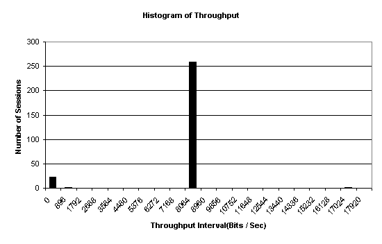
Figure 5.
Figure
5 shows that the many of the sessions had an average session throughput of 8064
bps. Below is a table showing the
average length and throughput of the sessions in the trace.
|
|
Length (bytes) |
Throughput (bits/sec) |
|
Average: |
934.75 |
7891.72 |
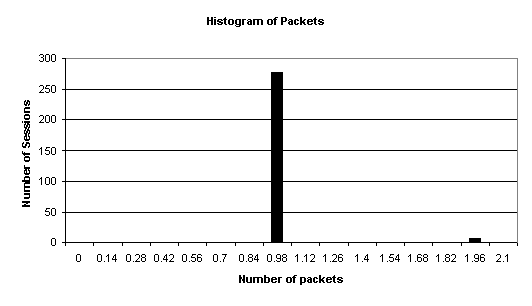 Next, the number of packets
per session are analyzed. In the
program, we keep a linked list of sessions opened during the trace. For each session, we count the number of
packets transferred. The following is a
histogram of the number of packets for the sessions.
Next, the number of packets
per session are analyzed. In the
program, we keep a linked list of sessions opened during the trace. For each session, we count the number of
packets transferred. The following is a
histogram of the number of packets for the sessions.
|
# sessions |
Packet count |
|
277 |
1 |
|
7 |
2 |
Figure 6
This
graph shows us that an overwhelming majority of the sessions only exchanged one
packet throughout the entire trace.
Seven sessions managed to exchange two packets. Since Telnet involves user interface, the
number of packets sent in a short interval, 0.94 seconds, will most likely be
small.
|
|
Number of Packets |
|
|
Average |
|
Because most sessions only exchanged 1 packet, the average number of packets in the trace is 1.0246.
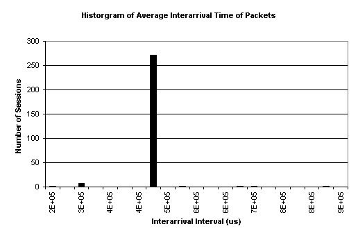 After measuring the packets
per session, we next found the packet interarrival time for each session. This was done by dividing the total session
duration by the packets in the session.
Specifically, there are three cases to consider. When both SYN and FIN bits are seen in the trace,
we divide the duration by the number of packets – 1. When only one is seen in the trace, we divide by the number of
packets. When neither SYN nor FIN are
seen, we divide by the number of packets + 1.
Figure 7 portrays the results of this experiment.
After measuring the packets
per session, we next found the packet interarrival time for each session. This was done by dividing the total session
duration by the packets in the session.
Specifically, there are three cases to consider. When both SYN and FIN bits are seen in the trace,
we divide the duration by the number of packets – 1. When only one is seen in the trace, we divide by the number of
packets. When neither SYN nor FIN are
seen, we divide by the number of packets + 1.
Figure 7 portrays the results of this experiment.
|
# sessions |
Interarrival time (us) |
|
1 |
224784 |
|
1 |
2243573 |
|
7 |
315948 |
|
271 |
473922 |
|
1 |
527692 |
|
1 |
684385 |
|
1 |
709413 |
|
1 |
890551 |
Figure 8
Many of the sessions have the same average packet interarrival time. This is probably due to the fact that for most of the sessions, we only see one packet, and we do not see a SYN or FIN bit. Therefore, when we calculate the average interarrival times, the values will be the same for most of the sessions. Below is a table of the average interarrival time.
|
|
Interarrival Time (us) |
|
Average |
471565.2 |
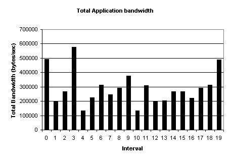
The last part of the project involves measuring the bandwidth of the Telnet application. Below is a plot of the bandwidth over the entire trace.
|
Application Bandwidth |
|
|
Interval |
|
|
0 |
491960.6685 |
|
1 |
201553.0047 |
|
2 |
268104.3214 |
|
3 |
577143.8217 |
|
4 |
133187.0358 |
|
5 |
223835.2465 |
|
6 |
312478.8994 |
|
7 |
246729.4058 |
|
8 |
290344.3619 |
|
9 |
377363.2681 |
|
10 |
134052.1607 |
|
11 |
310769.7502 |
|
12 |
199780.5537 |
|
13 |
204042.8764 |
|
14 |
269011.6475 |
|
15 |
267386.9007 |
|
16 |
222822.4173 |
|
17 |
291103.9838 |
|
18 |
311761.4787 |
|
19 |
489196.4889 |
|
Avg for Lifetime |
291130.186 |
Figure 9
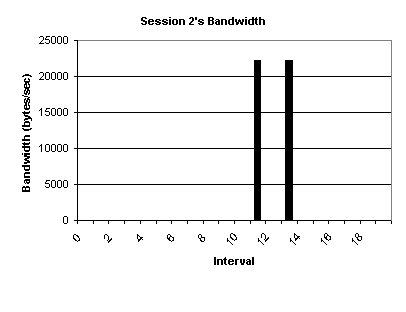
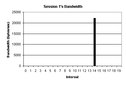 Next, five arbitrary sessions were picked from the
285 Telnet sessions in our trace. These
sessions were divided into 20 intervals, and their bandwidths over each
interval are plotted.
Next, five arbitrary sessions were picked from the
285 Telnet sessions in our trace. These
sessions were divided into 20 intervals, and their bandwidths over each
interval are plotted.
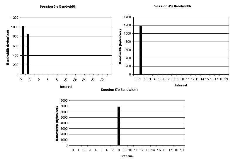
As we can observe, the TCP
protocol used more than the UDP protocol, and packet size for TCP is larger
than UDP, which is why there is three times more TCP packets, while TCP
occupies ten times more relative bandwidth than UDP.
When analyzing Telnet, we
obtained some unusual results. We
measured a total of 285 sessions in the trace.
Each session had about the same session length. Most of the sessions only transferred one
packet in the trace lifetime. Packet
interarrival time was also about the same for each session because almost every
session had the same duration (the trace lifetime) and the same number of
packets (1). Therefore, when graphing
the bandwidth of five random sessions over the trace lifetime, we see sparse
activity.
Due to the unusual results
of our trace, we decided to verify our packet analyzer program with other
traces. The results from these traces
did not seem as unusual. Hence, we believe,
our analyzer program functions properly, but our trace is abnormal.
We
also tried analyzing HTTP sessions in hopes of obtaining more typical
results. However, we found about 5,000
HTTP sessions in the trace. This would
not have been practical to use for this report.
|
|
||
|
Home | About Me | Text Depository | Future Enhancements | Guest Book | Links
All Rights Reserved. |