LX Flow Map: An Optimal Technology
Mapping Algorithm for Delay Optimization in LX Based FPGA Designs with Actually
Feasible Cuts
Michael Chen, Donald Lam, and Yu-Li Lin
Department of Computer Science
University of California, Los Angeles, CA 90095
{forbid,donaldl,yml}@cs.ucla.edu
Abstract
As the field programmable gate-array (FPGA) technology grows, faster, cheaper, and smaller circuits are being developed.� However, the fact that lookup-table (LUT) size increases in a polynomial order with respect to the number of inputs cannot be avoided by faster and smaller circuits.� While 4-LUTs are relatively cheap, 5-LUTs provide a broader set of circuits that can be represented at a higher cost.� To serve as a middle ground, we shall explore the LX-cell, a 4-LUT combined with an XOR gate.� The attractiveness of the LX-cell is the fact that it can represent a larger set of circuits than the 4-LUT with a minimal cost increase.� While the Flow Map technology mapping algorithm is Delay Optimal for conventional Lookup-Table Based FPGA Designs, it cannot take advantage of the extra functionality provided by the LX cell.� From the LX Flow Map Algorithm we can sometimes achieve the same depth as the 5-LUT Flow Map results.
1 �������� Problem Formulation and Definitions
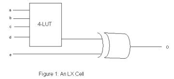
Suppose that a new FPGA uses a 5-input logic cell, named the LX cell, for implementing combinational logic.� Each LX cell consists of a 4-input look up table (4-LUT) whose output goes into a 2-input XOR gate (Figure 1).� The other input of the XOR gate is the 5th input to the LX cell.� To make efficient use of the LX cell we have developed a LX Flow Map algorithm.� Given a multi-level two-input circuit N, the algorithm can map it into a network N� of LX cells such that the depth N� is minimal and the number of cells used is minimized as a secondary objective.
2��������� LX Cell Cut generation
Our approach to finding a depth minimal LX Cell mapping of a given 2-input circuit is primarily based on the Flow Map algorithm.� To guarantee an optimal solution with respect to the Flow Map algorithm, we choose to exploit the fact that our solution should achieve a solution better than the 4-LUT mapping and no better than the 5-LUT mapping.� By using the existing Flow Map algorithm, we are able to establish candidates for 5-feasable cuts on a given network.� From the optimal 5-feasable cut candidate we shall test to see if the cut has 5 inputs (5-cut) or less than 5 inputs.� If the Flow Map returns a cut of less than 5 inputs, then we can simply represent it with the 4-LUT with a hard wired 0 for the fifth input to the XOR gate.�
2.1������ XOR Extraction
If the Flow Map algorithm returned a 5-cut as the depth minimal cut, then we need to test the network to see if the 5-cut network can actually be mapped to an LX cell, which shall be referred to as �actually feasible�.� Normally, we do not need to perform this check when trying to map 5-LUT cells because any 5-input network can be represented with a 5-input lookup table.� However, our LX cell cannot represent all 5 input networks.� It can only represent a circuit from which we can perform XOR extraction to.� This means we can represent the circuit as a 4-LUT XOR with one of the inputs, i.e.
f(x���1, x2, x3, x4,x5) = f(x���1, x2, x3,x5) � x4��������������������������������������������� (1)
2.1.1��� Actually Feasible
The XOR extraction is a two step approach.� First we have to figure out if an XOR can be extracted, and if so with which variable.� This is the actually feasible test.� We can test if a 5-cut is actually feasible by testing the 5 inputs one by one to see if it can be used to extract the XOR.� This is a simple and elegant test of the equivalence of the function�s cofactor with respect to the variable of interest with the complement of the negative cofactor of the function with respects to the same variable.
Lemma 1:
fx
= (fx�)� �
f(x���1,
x2, x3, x4, x) = f(x���1,
x2, x3,x4 ) � x�� ����������� ����������� (2)
Proof:
����������� f(a,b,c,d,e) = f(b,c,d,e) � a if and only if fa = (fa�)�
�if� proof:
����������� if �������� f(a,b,c,d,e)
= f(b,c,d,e) � a
����������� then
����������������������� if �������� a = 1
����������������������������������� f(1,b,c,d,e) = 1 � f(b,c,d,e)
�
fa =
1 * f�(b,c,d,e) + 0 * f(b,c,d,e) = f�(b,c,d,e)
����������������������� if �������� a = 0
����������������������������������� f(0,b,c,d,e) = 0 � f(b,c,d,e)
����������������������� �������� fa� = 0 * f�(b,c,d,e) + 1 * f(b,c,d,e) = f (b,c,d,e)
����������� �� fa = f�(b,c,d,e) = (fa�)�
�only if� proof
if �������� fa = (fa�)���������������������������������������������������������������������������������������������������������������������� f(a,b,c,d,e)
= a *� fa + a� *� fa������������������������������������������������������������������� (cofactor expansion)
����������� = a * (fa�)� + a� * fa�
����������� = a � fa�
����������� = a � f(b,c,d,e)
n
2.1.2��� Retrieve the Remaining 4-Input Function
Second, we must retrieve the resulting 4-input-function after the XOR has been extracted.� If one variable is actually feasible in step one of the XOR extraction method then we can extract the remaining 4-input function with one of the following two approaches:
Method 1:
Given that we can extract an XOR from the function with a known variable,
�f(a,b,c,d,e) = a � f(b,c,d,e)
we can extract the remaining function by applying an XOR to the same variable
f(a,b,c,d,e) �� a =
a �
f(b,c,d,e) � a
= f(b,c,d,e)
Method 2:
From the cofactor expansion in Lemma 1 we saw that fa = a � fa�
So, the negative cofactor, fa�, is the remaining function.
At this point the function can be mapped to the LX cell.� If, however, we failed on step 1 of the XOR extraction for all variables then we will repeat the process for the next best cut, testing the number of inputs and seeing if it�s actually feasible.
2.2������ Depth Minimal Cut Generation
To generate a list of cuts to consider, we choose to mimic the depth minimal cut generation algorithm presented in the Flow Map algorithm.� For every node, we shall generate a sub graph Nu representing the current node of interest, u, and all its predecessors from the original network.� Since the graph is visited in topological order from the inputs, it is guaranteed that all predecessors to the node of interest have already been processed.� From these sub-graphs we need to generate all depth minimal cuts of input size less than or equal to 5.� By definition, from the Flow Map algorithm, this is a division of the graph into two sections, where all the inputs are on the higher section, and the output (node of interest) is in the lower section.� This division in theory is placed across only nodes and not edges.� Unlike the strategy used in the Flow Map algorithm, we did not need to divide every node then label the connecting edge of weight 1, while labeling the original edges of weight infinity.�
2.2.1��� Equivalence of Cuts Generated By the Two
Algorithms
In our cut finding algorithm, we are still able to retrieve depth minimal cuts by searching from our node of interest the first set of nodes which do not have any interdependency, where one is not the predecessor of another.
Lemma 2:
A set of nodes define a depth minimal cut if and only if
none of the nodes are a predecessor of another.
Proof:
�if proof by contra positive�
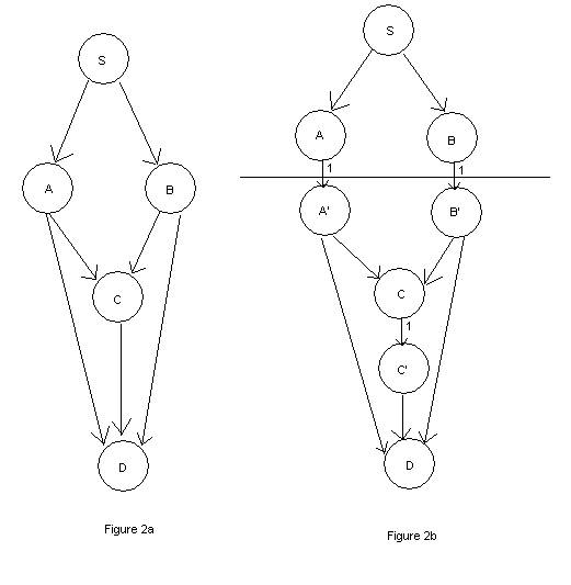
We want to show the contra positive: if at least one of the nodes is a predecessor of another, then the set of nodes do not define a cut.� Assume for the sake of contradiction that at least one of the nodes is a predecessor of another, and the set of nodes define a cut.� We can see from Figure 2a that in the set of nodes {A,B,C}, node C has node A and B as predecessors.� Furthermore, we can see from Figure 2b an intermediate result of the flow map algorithm, with the only cut shown.� Thus {ABC} cannot form a cut.� ��� if at least one of the nodes is a predecessor of another, then the set of nodes do not define a cut.� So, by the proof of the contra positive, if a set of nodes define a depth minimal cut then none of the nodes are a predecessor of another.
�only if proof by contra positive�
We want to show the contra positive: if the set of nodes do not define a depth minimal cut, then at least one of the nodes is a predecessor of another.� Assume for the sake of contradiction that the set of nodes do not define a depth minimal cut and none of the nodes is a predecessor of another.� We can see again from Figure 2a the set of nodes {B,C} are not predecessors of each other, yet Figure 2b shows that they do form a depth minimal cut.� �� Thus, If the set of nodes do not define a depth minimal cut, then at least one of the nodes is a predecessor of another.� From the contra positive, we see that if none of the nodes are a predecessor of another, then the set of nodes define a depth minimal cut.��
n
2.2.2��� Equivalent Drop Sets
Given a network N, we can run the cut finding algorithm on the only sink of the graph, and from the resulting cut node set we can recursively repeat the process to consider other cut sets by considering combinations of equivalent drop sets.� This will allow us to test every possible combination of nodes as a depth minimal cut.� A drop set is a set of nodes with the following properties: By dropping a node within an equivalent drop set, we will have to drop the whole set as an immediate consequence.� i.e. if two nodes, A and B, share a parent, C, then by dropping one node u, an element of {A,B}, we will have to add it's parents, set P, to our current cuts to test, but by property 1 we cannot have C �P and ū (complement of the set containing u, i.e. {A,B}-u) in the same cut set, since C is a parent of ū.
2.3
Cut Ranking
From the list of cuts, we can sort the set of cuts in best to worst order with the following criteria, where the best cut is defined as the one which guarantees the minimal depth and minimal number of LX cell usage in our original circuit.� We guarantee minimal depth by using a labeling system similar to that of the Flow Map algorithm.� While area minimization remains a secondary goal, we choose to model area minimization with a maximization problem of LX cell coverage of nodes.� While this model does not guarantee a minimal area, it does give a higher likelihood of choosing a cut that will reduce the over all area.� To distinguish between cuts according to depth we shall sort the list of cuts according to the maximum label of the nodes defining the cut.� The cut containing the minimum max label is the best one. From figure 3 we see:
|
Cut Name |
Node Labels |
Max Label |
Cut size |
Label Sum |
|
Cut 1 |
0,0,0,0,0 |
0 |
5 |
0 |
|
Cut 2 |
0,0,0,1 |
1 |
4 |
1 |
|
Cut 3 |
1,1,1 |
1 |
3 |
3 |
|
Cut 4 |
1,1,0,0 |
1 |
4 |
2 |
Table 1
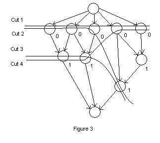
From the first sort criterion, it is obvious that Cut 1 is the best cut; however, since we have no idea if this 5-cut is actually feasible, we need to be able to distinguish between the other cuts.� Since all the other cuts have the same Max Label, an incorrect sort of the remaining cuts will affect only the area, but not the depth of our network.
����������� The next sort within our bucket (Cuts with the same max label) is by the cut size.� From this criterion, we see from Table 1 that Cut 2 and Cut 4 are indistinguishable from each other, yet clearly better than Cut 3.
����������� To distinguish between Cut 2 and Cut 4, we use the last criterion, minimization of the sum of the labels.� Since Cut 2 and Cut 4 have Label Sum 1 and 2 respectively, Cut 2 is better than Cut 4.� From the combined criteria we can see from best to worse the Cuts are 1,2,4,3.
2.4������ Labeling
To label nodes we shall use a method similar to the one described in the Flow Map algorithm.� A node will receive the same label as the max label of its parents.� If we can find an actually feasible cut from this node then the label stays the same.� Otherwise, increase the label by 1.
�
3��������� LX Cell Mapping
Once we have found the best cut available for every single node we are ready to map the LX cells on to the network.� To do this we start mapping from the primary outputs, where every primary output gets one cell.� Then from all the inputs of the cell, we repeatedly apply this process.� This is the same method used in phase 2 of the flow map algorithm.
4��������� Algorithms
Algorithm LXFlowMap
/*phase 1 label network and find cuts*/
for each PI node v do
����������� l(v) = 0
T= list of non-PI nodes in topological order
While T is not empty do
����������� Remove first node t from T
Cutlist(t)= LXCutlist(t)
For each cut C in Cutlist(t)
����������� C(maxlabel)= max(l(cv): cv is every node in C)
����������� C(cut size) = size of input(C)
����������� C(sum) = sum(l(cv): cv is every node in C)
����������� Bubble sort by maxlabel
����������� For each node with the same maxlabel bubble sort by cutsize
����������� For each bucket with the same max label and cutsize sort by sum
�����������
For each cut C in Cutlist(t)
If C is not actually feasible
����������� ����������� Remove C from Cutlist(t)
����������� End if
����������� If Cutlist(t) is empty
����������������������� l(v) =max(l(p) : p is the input to l) + 1
Else
����������������������� l(v) =max(l(p) : p is the input to l)
����������������������� Cut(t) = first element of Cutlist(t)
����������� End if
End while
/* phase 2 mapping */
L = list of PO nodes
While L contains non-PI nodes do
����������� Take a non-PI node v from L;
����������� Generate a K-LUT v� to implement the function of v
����������������������� Such that input(v�) = input (Cut(v))
����������� L = (L-{v}) U input (v�)
End while
End algorithm
Algorithm Cutlist(t)
ListofCuts
N� = sub network of all nodes which are predecessors of t
NodeofinterestList = every input of t
Findcuts(ListofCuts,NodeofinterestList)
End Algorithm
Algorithm Findcuts(ListofCuts,NodeofInterestList)
Change =0
While(change==0)
for every node n in NodeofinterestList
����������� if��������� n is a predecessor of x: every other node in NodeofinterestList
����������������������� Chang =1
����������������������� NodeofinterestList+= parents of n
����������������������� Nodeofinterest �=NodeofInterestList
����������� end if
end for
end while
if sizeod n odesofinterest <=5
LostofCuts +=nodesofinterest
End if
For every combination of nodes in the nodes of interest k,
����������� Findcuts(ListofCuts,k)
End for
End algorithm
5��������� Complexity Analysis
The critical section of our algorithm is the portion that finds the list of feasible cuts.� By attempting to generate all cuts of k=5 or less we have implemented an O(nk) cut generation algorithm, where n is the number of nodes in our network.
6��������� Results
|
Circuit |
C17 |
Small 1 |
Small 2 |
Frg2 |
|
Node |
6 |
26 |
78 |
797 |
|
Original Depth |
3 |
6 |
14 |
14 |
|
Flow Map 4 Depth |
1 |
3 |
6 |
6 |
|
Flow Map 4 Area |
2 |
11 |
38 |
492 |
|
LX Flow Map Depth |
1 |
1 |
3 |
5 |
|
LX Flow Map Area |
2 |
1 |
3 |
393 |
|
Flow Map 5 Depth |
1 |
1 |
3 |
4 |
|
Flow Map 5 Area |
2 |
1 |
3 |
426 |
|
Flow Map 5 & 4
Depth Difference |
0 |
2 |
3 |
2 |
|
Flow Map 5 & 4
Area Difference |
0 |
10 |
35 |
66 |
|
LX & Flow Map 4
Depth Difference |
0 |
2 |
3 |
1 |
|
LX & Flow Map 4
Area Difference |
0 |
10 |
35 |
99 |
|
LX & Flow Map 5
Depth Difference |
0 |
0 |
0 |
-1 |
|
LX & Flow Map 5
Area Difference |
0 |
0 |
0 |
33 |
Table 2
As we can see from Table 2 above, the LX mapping algorithm gives extremely competitive results for small circuits.� From the test circuits used we saw that there was no improvement in C17.� However this is due to the fact that there is no room for improvement between the Flow Map 4 and Flow Map 5 results.� On small 1 and small 2 however, there was room for improvement and between Flow Map 4 and Flow Map 5.� Our LX algorithm was able to match the Flow Map 5 results in both Area and Depth.� On Frg2, a much larger circuit, we begin to see a difference in depth between Flow Map 5, LX Flow Map, and Flow Map 4.� Here Flow Map 5 had a depth gain of 2 over Flow Map 4, but LX Flow Map was only able to achieve a gain of 1.� However, an interesting fact to note is that LX flow Map out performs Flow Map 5 in area minimization.� While Flow Map 5 has a 66 cell gain over Flow Map 4, LX Flow map as achieved a 99 cell gain over Flow Map 4.� This is a 50% gain increase and in some cases it may justify the 50% loss in depth gain.
To verify the results above please visit a server on cs.ucla.edu, in the directory ~donaldl/CS258G/LX-FlowMap-S/
Type my.x <blif name> to run the LX Flow Map program
on a given circuit described in the blif file.
7��������� Advantages and Limitations
During the construction of our program, we attempted to generate cuts via the Cut Enumeration Scheme.� It turns out that our algorithm ran faster than the Cut Enumeration version on smaller circuits.� The limitation to our algorithm is the high complexity.� This makes the run time on large circuits extremely high.� Our main advantage is that our algorithm guarantees the optimal solution.
8��������� Future Work
It is apparent that the execution time of our program is much slower than that of Flow Map.� The main reason should be due to implementation issues.� Some main areas that can use improvements are listed as follows:
9��������� References
1. J.Cong and Y. Ding, �FlowMap: An Optimal Technology Mapping Algorithm for Delay Optimization in Lookup-Table Based FPGA Designs�, IEEE Trans. on Computer-Aided Design, Vol. 13, No. 1, pp. 1-12, Jan. 1994
2. J. Cong, C. Wu, and Y. Ding, �Cut Ranking and Pruning: Enabling A General And Efficient FPGA Mapping Solution�, Proc. Of Int�l Symp. On Field-Programmable Gate-Arrays, Monterey, CA., Feb. 1999
3. Chapters 7, 8, and 10 of the textbook.
|
|
||
|
Home | About Me | Text Depository | Future Enhancements | Guest Book | Links
All Rights Reserved. |